Spot Tracking & Analysis for LEED (STAL)

Overview

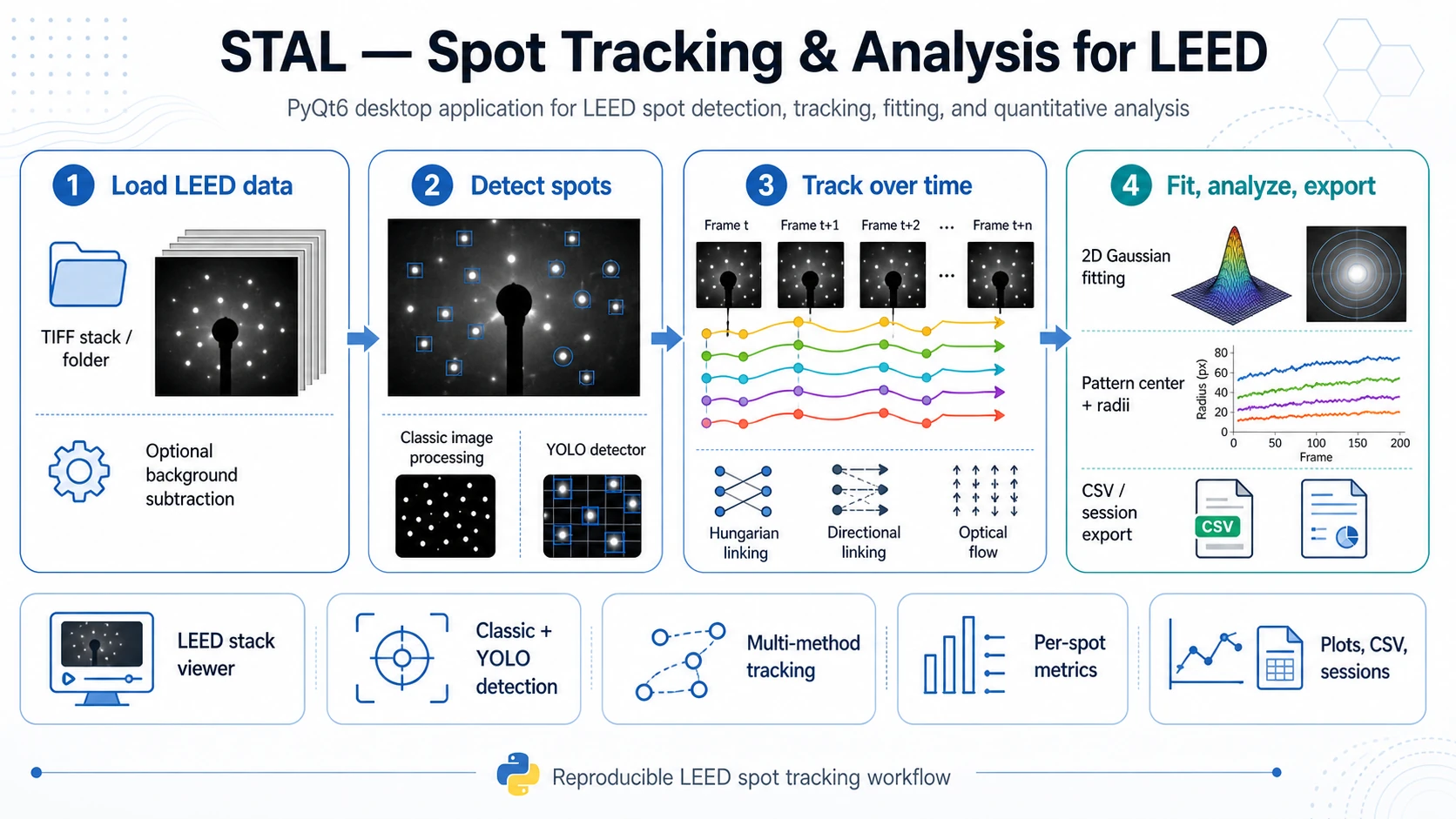
Spot Tracking & Analysis for LEED (STAL) (package name: trackleed) is a PyQt6 desktop application for analysing time-resolved LEED image sequences. It helps load LEED frames, detect diffraction spots, track spot motion across frames, refine spot positions with 2D Gaussian fitting and export quantitative results for downstream analysis.

The application is currently an active research and development tool. The stable baseline workflow is built around classical image processing, YOLO-based spot detection, detection linking with Hungarian assignment and Lucas-Kanade optical flow. The current development branch extends this baseline with a benchmarking-oriented tracker layer where multiple modern point, bounding-box and mask/video trackers can be tested against the classical YOLO + Hungarian and optical-flow workflows.

What STAL Does

STAL turns LEED image sequences into structured, reviewable and exportable spot trajectories. It is designed for experiments in which diffraction spots move, appear, disappear, dim, broaden, split or become difficult to follow manually.

Main capabilities include:

• loading LEED frame sequences from image directories,
• optional GIF import by sampling frames into PNG files,
• optional background loading and subtraction,
• masking of image regions that should not participate in detection or analysis,
• diffraction-spot detection with either a classical white-top-hat + peak-finding pipeline or a YOLO detector,
• manual ROI editing for correcting, adding, deleting or refining spot definitions,
• tracking across frames with classical and experimental tracker backends,
• 2D elliptical Gaussian fitting for every tracked spot ROI,
• pattern-center estimation and radius calculation relative to that center,
• per-track and per-frame metrics, plots, tables, overlays, CSV exports and JSON session persistence.

Typical Workflow

1. Load data - open a directory with LEED frames from File > Open Directory.... The parser accepts common LEED frame naming conventions and simpler numeric names such as 001.tif or frame_001.png.
2. Import or prepare frames - optionally import a GIF, load a background image and define masks for beam-stop areas, labels, detector artefacts or other ignored regions.
3. Detect spots - use the Find Spots panel. For robust baseline work, start with the classic detector and tune blur, white-top-hat radius, minimum distance, threshold and ROI size. For more complex datasets, use YOLO checkpoints.
4. Track over time - choose a tracking algorithm in the Tracking panel. Baseline options include Hungarian linking, directional Hungarian linking, Lucas-Kanade optical flow and skip-anchor optical flow.
5. Review and edit tracks - open the tracking visualizer to inspect trajectories, delete false tracks, add or move ROIs, merge tracks or retrack selected spots.
6. Run quantitative analysis - use Analyze Tracks to fit a 2D elliptical Gaussian to each tracked ROI. STAL stores fitted centers, amplitudes, widths, FWHM, asymmetry, volume, fit quality, radius from the pattern center and propagated errors when available.
7. Export and save - export CSV files, track overlay images, YOLO labels or complete sessions. Sessions preserve loaded files, spot definitions, masks, tracks, analysis results and selected settings.

Detection Methods

Classic Detector

The classic detector is a transparent image-processing pipeline intended as a reproducible baseline. It includes optional background normalization/subtraction, residual background estimation by Gaussian blur, white top-hat filtering, local-maximum detection and conversion of detected peaks into rectangular SpotROI objects.

This method is useful when the diffraction pattern is clean, spots are relatively separated and a reproducible non-ML baseline is needed.

YOLO Detector

The YOLO detector uses Ultralytics .pt checkpoints placed in tracking_models/yolo/. Detected boxes are converted into SpotROI objects and can then be tracked, edited, analyzed or exported as YOLO labels.

YOLO is useful when spots vary strongly in contrast, when background artefacts make threshold-based detection unstable or when the user wants to build and iterate an annotated LEED detection dataset.

Tracking Methods and Development Status

STAL supports a layered tracking strategy. Classical methods provide a reproducible baseline, while experimental tracker integrations make it possible to compare modern video/object tracking methods on the same LEED data.

Baseline Tracking

• Detection Linking / Hungarian - links per-frame detections by distance-based assignment.
• Directional Linking - radial-aware Hungarian linking with lateral penalties, ring-bin gating, dynamic maximum distance, optional direction flip handling and track-gap tolerance.
• Lucas-Kanade Optical Flow - sparse optical flow from a selected reference frame.
• Optical Flow with skip-anchor logic - a more robust LK variant with optional forward-backward checks, NCC checks, centroid refinement and gap handling.

Experimental Tracker Layer

The repository includes a registry-based tracker architecture with point, bounding-box and mask/video backends. These integrations are intended for benchmarking and method development, especially on difficult LEED sequences with dim, blurred, moving or temporarily disappearing spots.

Tracker family	Backends present in the repository	Typical use
Point trackers	TAPIR, BootsTAPIR Online/Causal, LocoTrack, CoTracker3, TAPNext, Track-On-R, PIPs++, MFTIQ	Following selected spot centers as points across frames.
Bounding-box trackers	ToMP/TaMOs, OSTrack	Tracking spot ROIs as object boxes and converting the result to representative spot positions.
Mask/video trackers	SAM2, SAMURAI, DAM4SAM, DEVA, Cutie, XMem2	Propagating masks or segmented spot regions and extracting a representative point such as mask centroid, peak-in-mask or Gaussian-in-mask.

Not every backend is equally mature or equally easy to install. Some require an upstream repository, model checkpoints, CUDA-compatible PyTorch builds or a dedicated Conda/Python environment. External tracker integrations should therefore be treated as experimental benchmarking backends unless validated on the target dataset.

Subprocess-Based Tracker Execution

Several modern tracking libraries have dependency stacks that are difficult to install in the same Python environment as the main PyQt6 application. STAL therefore supports a subprocess mode for many backends. The main application remains in its normal environment, while a selected tracker runs in a separate Python interpreter, often from a dedicated Conda environment.

Typical setup pattern:

python -m venv .venv
source .venv/bin/activate  # Windows: .venv\Scripts\activate
pip install -r requirements.txt
python -m trackleed

For external tracker backends, the GUI can be configured with the external repository path, dedicated Python executable, checkpoint/model directory and backend mode: direct or subprocess.

Quantitative Outputs

After tracking, STAL can run a Gaussian-based analysis pipeline. For each tracked spot and frame, it can compute:

• fitted global center coordinates,
• Gaussian amplitude and offset,
• sigma_x, sigma_y and orientation angle,
• FWHM X/Y and corresponding errors,
• integrated Gaussian volume and volume error,
• asymmetry,
• R-squared and reduced chi-squared,
• radius relative to the pattern center,
• radius error when center and fit errors are available.

Pattern-center modes include per-frame estimation, circle fitting, ellipse fitting, global median center, temporal center smoothing and manually defined circle or ellipse overlays. Frame-level summaries include average radius per frame and standard error across tracks.

Positions Analysis

In addition to standard track analysis, STAL includes a positions-analysis workflow for grouped tracks. A user can define groups consisting of one reference track and one or more satellite tracks. The tool then refits positions frame-by-frame and reports relative geometry: reference and satellite fitted centers, dx, dy, radial distance r, fit-quality status, validation flags, grouped CSV outputs and overlay images.

This mode is useful when the scientific question depends on relative spot positions rather than only absolute motion or radius from the global pattern center.

Use Cases

• tracking LEED pattern evolution during an experiment,
• comparing tracking algorithms on difficult LEED data,
• building and improving YOLO spot detectors,
• quantifying per-spot shape and fit quality,
• measuring relative satellite/reference spot geometry,
• preparing reproducible figures, tables, overlays and sessions.

Input and Output

Input

• directories with LEED image frames,
• .tif, .tiff and .png files as primary directory inputs,
• GIF import via frame extraction,
• optional background image,
• optional model checkpoints for YOLO and external tracker backends,
• optional filename metadata for element, surface, frame/time, temperature, energy and coverage.

Output

• full_analysis_per_spot.csv - per-track, per-frame Gaussian fit and derived metrics,
• pattern_center_data.csv - pattern-center data per processed frame,
• average_radius_per_frame.csv - frame-level radius summaries,
• track_legend.csv - track identifiers and starting positions,
• track_visualizations/ - PNG overlays with track traces,
• grouped positions-analysis CSV files and overlay images,
• YOLO labels and images for dataset building,
• JSON session files for saving and restoring the analysis state.

Installation

git clone <repository-url>
cd trackleed-2704-samurai
python -m venv .venv
source .venv/bin/activate  # Windows: .venv\Scripts\activate
pip install -r requirements.txt
python -m trackleed

Core dependencies include NumPy, SciPy, scikit-image, OpenCV, Matplotlib, Pandas, Pillow, tifffile, imageio, PyQt6, pyqtgraph, PyOpenGL, Ultralytics, PyTorch and TorchVision. For GPU-accelerated YOLO or experimental tracker backends, install a PyTorch build compatible with the local CUDA setup and prepare the required upstream repositories and checkpoints.

Scope and Limitations

STAL is intended for research workflows where visual inspection and validation remain important. The application can automate a large part of LEED spot analysis, but difficult datasets still require parameter tuning and manual review.

Important limitations:

• advanced tracker integrations are under active development and should be validated against the classical baselines,
• external trackers may require separate installation procedures, repositories, checkpoints, CUDA versions or subprocess execution,
• rich metadata such as temperature, energy and coverage depends on filename conventions,
• Gaussian-derived metrics are meaningful only when the fitted ROI actually contains a suitable spot and the fit quality is acceptable,
• tracking results should be inspected when spots cross, disappear, split, saturate or overlap with artefacts.

License

The project is distributed under the MIT License.